MIPLearn/docs/benchmark.md

Benchmarks

Using BenchmarkRunner

MIPLearn provides the utility class BenchmarkRunner, which simplifies the task of comparing the performance of different solvers. The snippet below shows its basic usage:

from miplearn import BenchmarkRunner, LearningSolver

# Create train and test instances
train_instances = [...]
test_instances  = [...]

# Training phase...
training_solver = LearningSolver(...)
training_solver.parallel_solve(train_instances, n_jobs=10)
training_solver.save_state("data.bin")

# Test phase...
test_solvers = {
    "Baseline": LearningSolver(...), # each solver may have different parameters
    "Strategy A": LearningSolver(...), 
    "Strategy B": LearningSolver(...),
    "Strategy C": LearningSolver(...),
}
benchmark = BenchmarkRunner(test_solvers)
benchmark.load_state("data.bin")
benchmark.fit()
benchmark.parallel_solve(test_instances, n_jobs=2)
print(benchmark.raw_results())

The method load_state loads the saved training data into each one of the provided solvers, while fit trains their respective ML models. The method parallel_solve solves the test instances in parallel, and collects solver statistics such as running time and optimal value. Finally, raw_results produces a table of results (Pandas DataFrame) with the following columns:

• Solver, the name of the solver.
• Instance, the sequence number identifying the instance.
• Wallclock Time, the wallclock running time (in seconds) spent by the solver;
• Lower Bound, the best lower bound obtained by the solver;
• Upper Bound, the best upper bound obtained by the solver;
• Gap, the relative MIP integrality gap at the end of the optimization;
• Nodes, the number of explored branch-and-bound nodes.

In addition to the above, there is also a "Relative" version of most columns, where the raw number is compared to the solver which provided the best performance. The Relative Wallclock Time for example, indicates how many times slower this run was when compared to the best time achieved by any solver when processing this instance. For example, if this run took 10 seconds, but the fastest solver took only 5 seconds to solve the same instance, the relative wallclock time would be 2.

Saving and loading benchmark results

When iteratively exploring new formulations, encoding and solver parameters, it is often desirable to avoid repeating parts of the benchmark suite. For example, if the baseline solver has not been changed, there is no need to evaluate its performance again and again when making small changes to the remaining solvers. BenchmarkRunner provides the methods save_results and load_results, which can be used to avoid this repetition, as the next example shows:

# Benchmark baseline solvers and save results to a file.
benchmark = BenchmarkRunner(baseline_solvers)
benchmark.load_state("training_data.bin")
benchmark.parallel_solve(test_instances)
benchmark.save_results("baseline_results.csv")

# Benchmark remaining solvers, loading baseline results from file.
benchmark = BenchmarkRunner(alternative_solvers)
benchmark.load_state("training_data.bin")
benchmark.load_results("baseline_results.csv")
benchmark.parallel_solve(test_instances)

Benchmark problems

MIPLearn provides a selection of random instance generators for some fundamental discrete optimization problems, as well a baseline MIP and ML formulation for these problems. The included problems are the following:

• Maximum Weight Stable Set Problem: Given a graph G=(V,E) with vertex weights, the problem is to find a maximum weight stable set of the graph, where a stable set is a subset of vertices, no two of which are adjacent. The class MaxWeightStableSetGenerator can generate random instances of this problem with specified probability distributions for number of vertices, edge probability and weights.

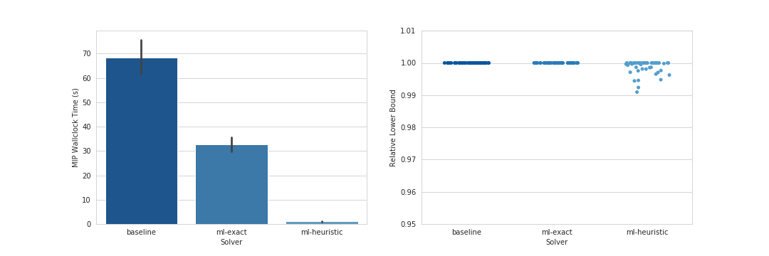
Benchmark results

To illustrate the performance benefits of MIPLearn, we present a small number of computational results for some of the included benchmark problems. For more detailed computational studies, see the references below. We compare three solvers:

• baseline: Gurobi 9.0 with default settings (a conventional state-of-the-art MIP solver)
• ml-exact: LearningSolver with default settings, using Gurobi 9.0 as internal MIP solver
• ml-heuristic: Same as above, but with mode="heuristic"

The experiments were performed on a Linux server (Ubuntu Linux 18.04 LTS) with Intel Xeon Gold 6230s (2 processors, 40 cores, 80 threads) and 256 GB RAM (DDR4, 2933 MHz). All solvers were restricted to use 4 threads, with no time limits, and 10 instances were solved simultaneously at a time.

Maximum Weight Stable Set Problem

• Fixed random graph (200 nodes, 5% edge probability)
• Random vertex weights ~ U(100, 150)
• 300 training instances, 50 test instances